Homework Assignments

ECEN/MAE 3723 Dynamic Systems

1. Plot the following complex numbers and put them in polar form.

• 1 + j3

• -1 - j3
• 1 - j3
• -1 + j3

• Find x + y in both rectangular form and polar form
• Find xy in both rectangular form and polar form

1. Find the transfer function for the following differential equation, and also solve the equation.

2.  B2.1, B2.2, B2.5, B2.6, B2.13 

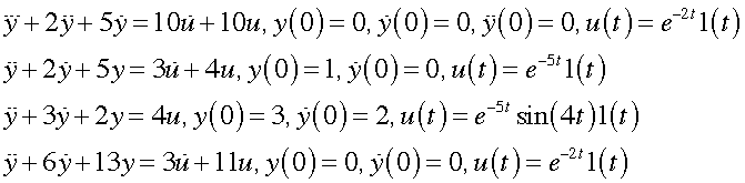
1. Find the transfer functions for the following differential equations, and also solve the equations.

2. Explain how the poles of the transfer function affect the time response.

1. Read the Laboratory/Project Handout, send me the names of your lab team, and order the Arduino Mega 2560 microcontroller that you will need for the first experiment.

1. For each of the following differential equations, a) find the transfer functions, b) find the system poles, c) write out the form of y(t) as specifically as you can, without performing any more calculations, d) find Y(s), e) find y(t).

2. B3.3, B3.4, B3.13, B3.14, B3.15, B4.4

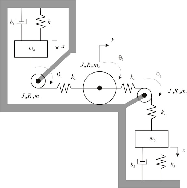
3. For the system in Figure 5-48, write out the equations of motion, and then find the transfer function (and the system poles) between the input u and the response z1. Describe the time response z1(t) in as much detail as possible, without any further equations.

4. In problem B.3.13, suppose J =1, b=1 and k=100.  Find the transfer function and the system poles. Describe the system response in as much detail as possible, without any further calculations.  If the system is initially at equilibrium and the input angle is a unit step, find the angle of the mass as a function of time.  Check your answer by using the MATLAB step command to find and plot the response.

1. B3.16, B3.17, B3.18, B4.6, B4.11, B4.17

2. Find the equations of motion for the following systems.

1. Order the motor shield, female barrel jack power connector, and the power supply that you will need for the second experiment. I will supply you with the DC motor in class on September 15.

---

Homework #6

Due Thursday Sep. 24

1) Differential Equations

2) Write out the equations of motion for this system. Write out all of the equations that you would need in order to solve, but do not perform any algebra.

3) B6.4, B6.5, B6.6, B6.7, B6.8, B6.15

---

Homework #7

2) B6.15, B6.16, B6.17, B6.18 (For analogies, try force-voltage and force-current, where possible.)

---

Homework #8

1. B7.2, B7.3, B7.4, B7.6, B7.7 (For all problems, use the across-variable of pressure, as discussed in class, instead of head.)

2. In problem B7.2, assume that the density of the fluid is 1.0E3 Kg/m3.  Find the pressure at the bottom of the tank as a function of time.

Homework #9

Due Thursday October 22

---

Homework #10

Due Thursday October 29

1. Problems B8.1, B8.2, B8.3, B8.4, B8.5, B8.6 (Use step inputs, if problem says to use a pulse inputs.) Select numerical values for the system parameters (e.g., resistors, capacitors, masses, etc.), find the pole locations and sketch each time response.

2. Discuss the relationship between the pole locations and the system time responses for each problem in 1.

3. Use the MATLAB command "step" to find and plot the step responses for each problem in 1, using the numerical values you selected.  Compare with your plots in 1.

---

Homework #11

Due Thursday November 5

1. Part I

2. Develop a model (differential equation) of an electrical circuit with an inductor, resistor and capacitor in series with a voltage source. The input to the system is the voltage source, and the output is the voltage across the capacitor. Find the transfer function.

3. Run simulations of the model in 2, with a unit step voltage source, using the step command in MATLAB, and the following values: L=1, R=3, C=0.5, and L=1, R=0.1, C=0.5, and plot the responses.

4. Find the pole locations in part 3, and show how the poles determine the time response (settling time, percent overshoot, frequency of oscillation, time of peak).

5. Compare your theoretical predicted settling time, percent overshoot, frequency of oscillation, time of peak (based on pole locations) with the values obtained from your simulation plots.  Discuss similarities and differences.

5. Problems B8.7, B8.8, B8.12, B8.13, B8.14, B8.15.  For each problem, find the pole locations, and describe how they affect the time response.